Installation and Run Instructions
Code Distribution Download
The CLEDB coronal field inversion code distribution is publicly hosted on Github:
https://github.com/arparaschiv/solar-coronal-inversion
To create a local deployment, use the git clone function:
git clone https://github.com/arparaschiv/solar-coronal-inversion
CLEDB_BUILD can utilize:
CLE precompiled GNU compatible Fortran binary executable files to generate databases. The module is run by utilizing a Bash script that enables parallel runs of serial computations. Binaries for both Darwin and Linux architectures are provided. More details are found in the CLEDB_BUILD - Database Generation module.
or
PyCELP python script to generate databases. This module is executed by running the python script with the same basic configuration as CLE. Parallelization is enabled. No binaries are required, but the PyCELP and CHIANTI databases need to be locally installed. The database build readme provides basic instructions on how to build a pycelp database. For simplicity, a precompiled database can be downloaded using the link in the main readme.
PyCELP database building requires the instalation of the respective package from git:
conda activate CLEDBenv
git clone https://github.com/tschad/pycelp.git
cd pycelp
python setup.py develop
Extended instructions can be found in the ‘PyCELP <https://github.com/tschad/pycelp.`_ repository.
Note
The CLE FORTRAN and PyCELP source codes are not included in this package. These are hosted in a separate repositories https://github.com/tschad/pycelp and https://github.com/arparaschiv/coronal-line-emission.
A CLEDBenv Python Environment
The CLEDB_PREPINV and CLEDB_PROC modules of CLEDB are written in Python.
The Anaconda environment system is utilized. Anaconda documentation and installation instructions can be found here.
We provide a configuration file CLEDBenv.yml to create a custom Anaconda environment that groups the CLEDB utilized Python modules briefly described above.
name: CLEDBenv
channels:
 - defaults
 - numba
 - conda-forge
dependencies:
 - python  = 3.13
 - numpy   = 2.1
 - numba   = 0.61
 - scipy   = 1.15
 - astropy = 7.0
 - pyyaml           ## 6.0.2 used only in ctrlparams for NUMBA global options
 - ipython          ## 8.34
 - ipympl           ## 0.96
-  tqdm             ## 4.67
 - jupyter          ## 1.1.1
 - jupyterlab       ## 4.3.5
 - matplotlib       ## 3.10.0
# - pytest           ## 8.3.5  ## necesary only for unit testing.
# - sphinx=8.2.3           ## 5.0.2  Not required by CLEDB; used only to build the documentation locally; see more in docs/requirements.txt
# - myst-parser=4.0.1      ## 0.18.1 Not required by CLEDB; used to add markdown parsing to documentation building.
# - sphinx-rtd-theme=3.0.2 ## 1.1.1 Not required by CLEDB; theme for the documentation


## please reflect any changes to pyproject.toml dependencies.
The configuration file is used to configure the required and optional CLEDB Python packages. In a terminal session you can create the environment via:
conda env create -f CLEDBenv.yml
After installing all packages the environment can be activated via
conda activate CLEDBenv
The user can return to the standard Python package base by running
conda deactivate
If dependency problems arise for any reason, CLEDBenv can be deleted and recreated with the default fixed-version packages from CLEDBenv.yml.
conda remove --name CLEDBenv --all
Danger
The CLEDBenv anaconda environment installs specific version packages. Cross-compatibility is verified by us. This feature ensures additional codebase stability. Updating the individual Python packages inside the CLEDBenv environment is not recommended and might break code functionality.
Basic Run Example
Move to the CLEDB working directory
cd ./solar-coronal-inversion
Databases can be built with:
./CLEDB_BUILD/rundb_1line.sh
See detailed database build instructions via the dedicated README-RUNDB found in the CLEDB_BUILD directory.
Two examples of running the full inversion package (assuming databases are already built) are provided as Jupyter notebooks and/or lab sessions.
./jupyter-lab test_1line.ipynb
./jupyter-lab test_2line.ipynb
Attention
Script versions for test_1line and test_2line are also available. These are tailored to be used in headless runs.
Headless Slurm Runs Overview
A few optimizations and modifications are provided in order to ensure a straightforward run of CLEDB on headless systems like research computing clusters. The Slurm environment is utilized.
Namely:
Instructions for resource allocation, installing, and running the inversion in both interactive and batch modes of Slurm research computing setups are provided.
The database building bash script has a dedicated headless version, rundb_1line_slurm.sh, where user options are hard-coded.
Pure python test scripts (test_*.py) are exported/generated from the Jupyter notebooks (test_*.ipynb) to be compatible with batch allocations.
A dedicated readme covering this topic can be consulted here or as standalone in the main CLEDB directory. The instructions are provided following the templates set by the Colorado University Research Computing User Guide.
Example Datacubes
A number of examples are included to help a user get started with inverting coronal fields with CLEDB. The test jupyter or python scripts will load different datafiles corresponding to one selected test case. Some cases are not yet fully implemented or available. The available datafiles can be donwloaded from the links below, or by following the Readme.md instructions. The Readme.md file also contains a method for downloading the data using only the terminal for headless systems.
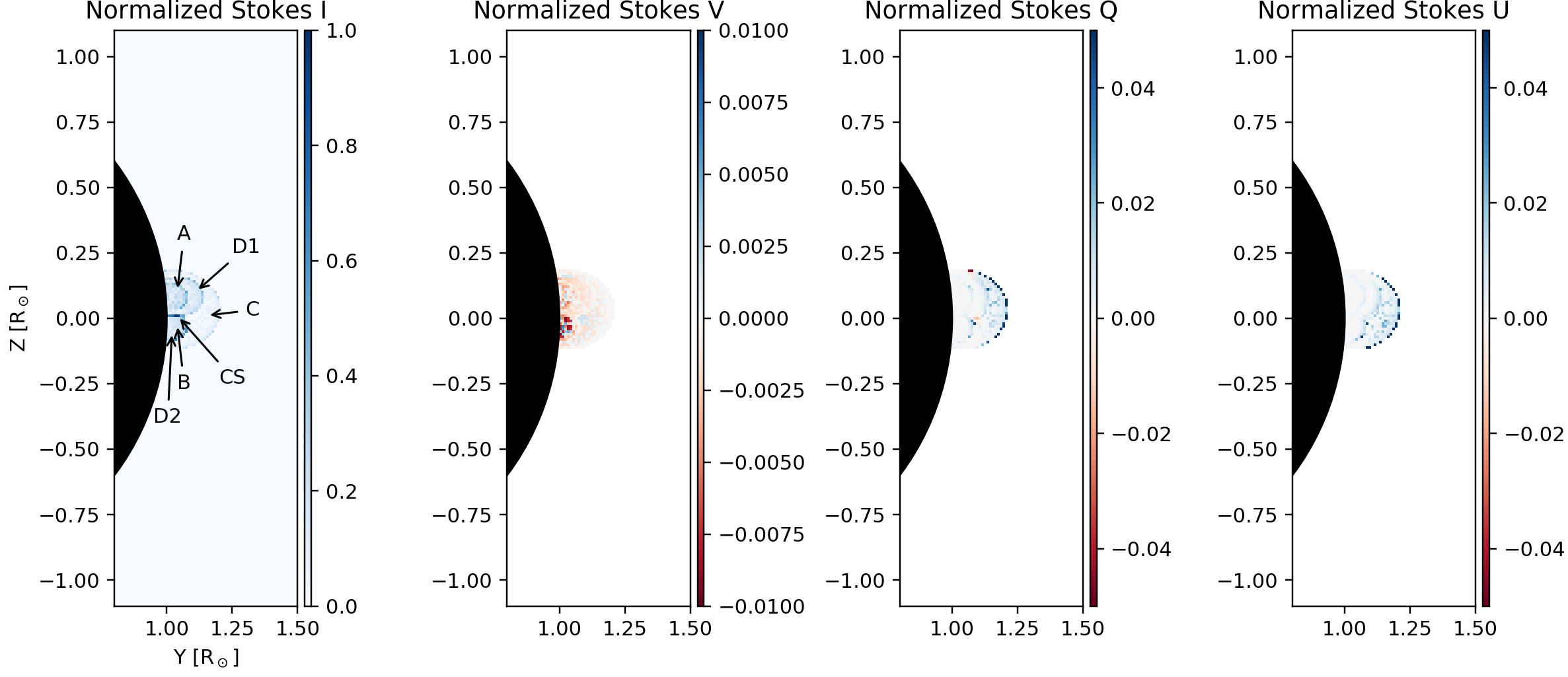
- 1.a CLE IQUV test example
Full Stokes synthetic IQUV data to test CLE generated databases. A CLE <https://github.com/arparaschiv/coronal-line-emission> computed forward-synthesis of Fe XIII 1074 and 1079 nm lines using a dipole generator program (See CLE dipolv.f). Three independent magnetic dipoles are generated at different positions along the LOS. These outputs are combined into a single LOS projected observation.
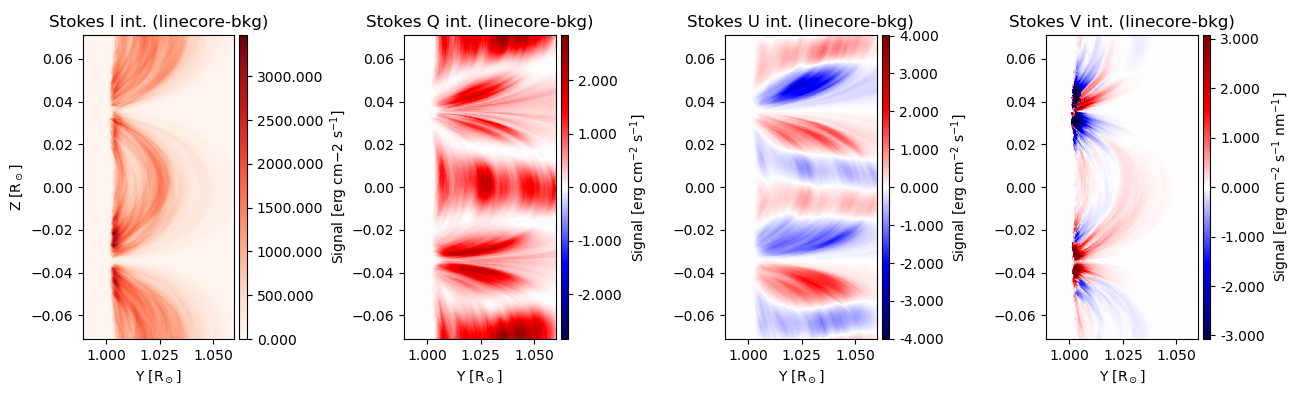
- 2.a PyCELP and MURAM IQUV test example
Full Stokes IQUV data to test PyCELP generated databases. A MURAM simulation of a dipolar structure at the :term`POS`. Fe XIII forward-synthesis via PyCELP. This synthetic observation was analyzed and described by Schad & Dima, SolPhys, 2021. This is a large datafile.
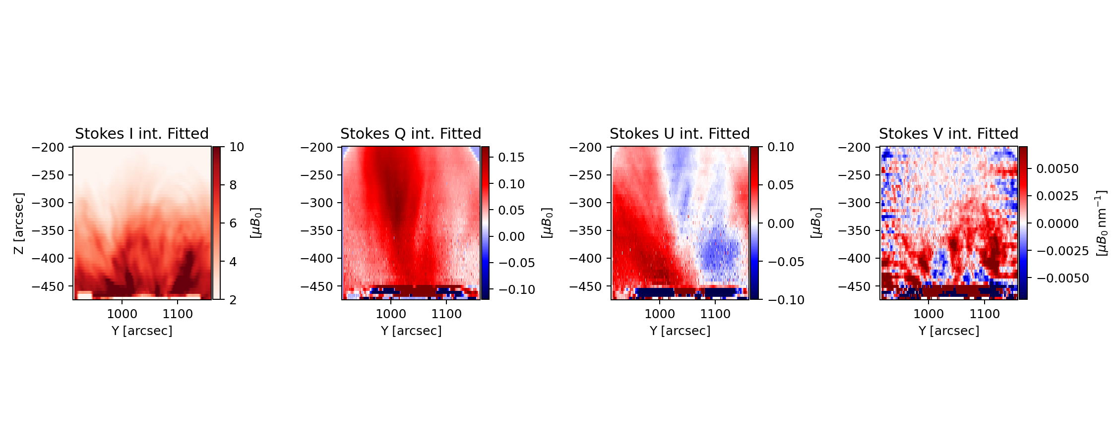
- 3.a DKIST Cryo-NIRSP integrated data test example.
Full Stokes line-integrated IQUV data. This example utilizes a real observation from DKIST Cryo-NIRSP from on March 23 2024. A preliminary processed observation of spectro-polarimetric Stokes IQUV measurements.
Caution
The 3.a datafiles are line-integrated IQUV datasets resulting from the analysis tutorial processing provided by the DKIST Science team. The data and analysis code can be found here This processing is just a conceptual example of analysis steps and not a careful science-ready processing. Neither the input data nor the output CLEDB products are scientifically validated and science ready.
Important
Processing of full spectro-polarimetric DKIST data is not yet included in CLEDB due to the complexities of manually tuning the processing of each dataset. It is recommended that you pursue an analysis following the steps described in the public DKIST Cryo-NIRSP tutorial linked above, and then feed the resulting integrated Stokes IQUV profiles after accounting for the photosphere, tellurics, crosstalk, and interference fringes.
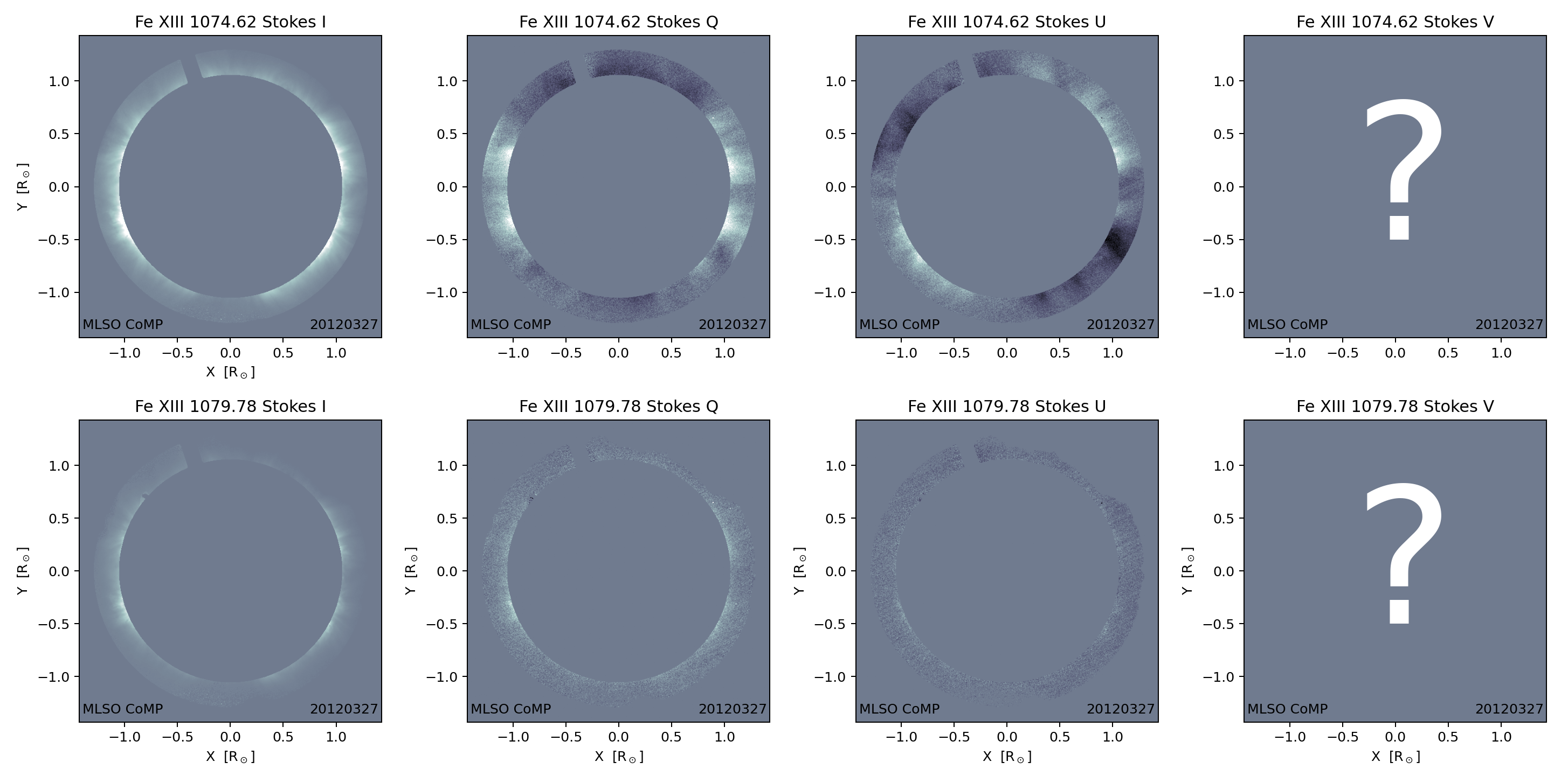
- 4.a CoMP IQUD only test example
Stokes IQU data. No Stokes V. This example utilizes a real observation from CoMP from on March 27 2012. CoMP is not capable of routinely measuring Stokes V. uCoMP ingestion is also implemented in CLEDB. Multiple real-life coronal structures are observed. Because Stokes V is not measured, we do not get access to an analytical solution via the BLOS_PROC module.
The IQU data can be downloaded from gdrive. This doppler data can be downloaded from gdrive.
- 4.b Doppler oscillation analysis results for data in 4.a
This is the additional data that needs to be brought in for obtaining a vector magnetic solution for the CoMP/uCoMP observation offered as part of the 4.a example. This data and methods of inferring POS magnetic maps from Doppler oscillations are described in Morton et. al, NatComm 2015 and Yang et. al, Sci. 2020. We utilize
sobs_dopp[:,:,0]that encodes the magnetic field strength and the wave angle derived from the Doppler oscillation analysis. The three other dimensions represent POS projections of the magnetic field. These are not currently utilized. The test_2line scripts will just create an empty array when a full Stokes IQUV inversion is requested, as in the 1. - 3. examples.
Note
For all IQUV examples, a user should expect solutions that are degenerate in pairs of two with respect to the LOS position. These need to be properly disambiguated for each observation. An additional analysis of the inversion outputs and decision is required.
Note
In the case of the IQUD example, a user should expect solutions that are degenerate in pairs of four with respect to the LOS position and the magnetic polarity. Currently, a more degenerate solution is retrieved when compared with the full Stokes IQUV inversions. Solutions to further disambiguate IQUD results are currently being trialed. Noteworthy is the fact that the two degeneracies (LOS position and magnetic polarity) are independent with respect to how the problem is posed. Thus, a selection of solutions should not be made as x in set [0,1,2,3] but as x in [1,4] or [2,3] solution subsets for an observed pixel. As mentioned above, these solutions need to be properly disambiguated for each observation. A manual analysis and decision is required.
Hint
A mapping of the magnetic field strength can be obtained from any of the IQUV test 1. - 3. cases. These alongside a calculation of the linear polarization azimuth can be fed as a sobs_dopp observation in a IQUD inversion scheme applied to the same test data or particular observations. (CLEDB will ignore the Stokes V information in this case). A set of four degenerate solutions will be obtained. One subset of two solutions will be geometrically identical to the full IQUV inversion output.