Input Variables and Parameters
Input Data and Metadata
header *keysSet of input header metadata information that should describe the
sobs_invariable. Expected keywords with simplified naming are detailed in this section. Detailed keyword information can be found for DKIST observations in the SPEC_0214 documentation and the uCoMP documentation .*keys to crpixn [] intReference pixel along x y or w (wavelength) direction.*keys to crvaln [] floatCoordinate value at crpix along x y or w (wavelength) direction.*keys to cdeltn [] floatSpatial (x,y) or spectral (w) platescale sampling along a direction.*keys to linpolref [] float(0, 2\({\pi}\)) range; Direction of database reference for the linear polarization.linpolref= 0 implies the direction is corresponding to a horizontal axis, analogous to the unit circle reference. Direction is trigonometric. The units are in radians. This is controlled via ctrlparams.*keys to instwidth [] floatMeasure of the utilized instrument’s intrinsic line broadening coefficient. The units are in nm. This is controlled via ctrlparams.*keys to nline [] intNumber of targeted lines; CLEDB can accept 1-line or 2-line observations.*keys to tline [:12, nline] string arrayString array containing the name of lines to process. Naming convention follows the database directory structure defined as part of theCLEDB_BUILDmodule.*keys to xs/naxis1 [] intPixel dimension ofsobs_inarray along the horizontal spatial direction.*keys to ys/naxis2 [] intPixel dimension ofsobs_inarray along the vertical spatial direction.*keys to ws [] intPixel dimension ofsobs_inarray along the spectral dimension.*keys to linpolref [] floatUsually points to a control parameter defining the orientation reference for linear polarization.*keys to instwidth [] floatIf instrumental width can be quantified and is significant, it gets recorded in this variable.
*keys to hpxycoords [] fltarrHeader metadata is fed to the WCS system to compute the spatial map of a slit raster observation.
*keys to wlarr [] fltarrHeader metadata is fed to the WCS system to compute the spectral dispersion coefficients of a slit.
keyvals [17] list of header variablesPacking of nx, ny, nw, nline, tline, crpix1, crpix2, crpix3, crval1, crval2, crval3, cdelt1, cdelt2, cdelt3, linpolref, instwidth, hpxycoords, wlarr in a list container to more easily feed the necessary keywords and fitted axes to other modules and/or functions.
sobs_in [nline][xs,ys,ws,4] float array; nline = 1 || 2 for (1-line) or (2-line)sobs_inis passed as a numba typed list at input. Data are input Stokes IQUV observations of one or two lines respectively. The list will be internally reshaped as a numpy float array of [xs,ys,ws,4] or [xs,ys,ws,8] size.
Ctrl. Parameters ctrlparams.py Class
# -*- coding: utf-8 -*-
# """
# @author: Alin Paraschiv
# """

class ctrlparams:
    """
    A set of inversion controlling parameters grouped in a convenient class that is passed along to inversion modules.

    To load the class:
    $par=ctrlparams()
    $print(vars(par))
    $print(a.__dict__)
    """
    def __init__(self):
        """
        Class only performs a main initialization for all variables.
        """
        ## General params
        self.dbdir        = './CLEDB_BUILD/'                                                   ## directory for database
        self.lookuptb     = self.dbdir + 'chianti_v10.1_pycelp_fe13_h99_d120_ratio.npz'        ## CHIANTI density look-up table
        self.verbose      = 1                                                                  ## verbosity parameter
        self.ncpu         = 100                                                                ## Number of cpu cores to use. If more than the available cores are requested, n-2 available cores are used.

        ## Used in CLEDB_PREPINV
        self.integrated   = False                                                              ## Boolean; parameter for switching to line-integrated data such as CoMP/uCoMP/COSMO
        self.dblinpolref  = 0                                                                  ## Parameter for changing the database calculation linear reference. Should not need changing in normal situations. radian units.
        self.instwidth    = 0                                                                  ## Parameter for fine-correcting non-thermal widths if instrument widths are known or computed by user. nm units.
        self.atmred       = False                                                              ## Parameter that controls whether to reduce photospheric and atmospheric contributions using spectral atlases. Useful for Cryo-NIRSP L1 data.

        ## Used in CLEDB_PROC
        self.nsearch      = 8                                                                  ## number of closest solutions to compute
        self.maxchisq     = 1000                                                               ## Stop computing solutions above this chi^2 threshold
        self.gaussfit     = 2                                                                  ## Gaussian parametric fitting to use instead of the standard CDF fitting
        self.bcalc        = 0                                                                  ## control parameter for computing the B magnitude for two line observations.
        self.reduced      = False                                                              ## Boolean; parameter for reduced database search using linear polarization azimuth
        self.iqud         = False                                                              ## Boolean; parameter for IQU + Doppler data matching when Stokes V is not measurable

        ##Numba jit flags
        self.jitparallel  = False                                                              ## Boolean; Enable or disable numba jit parralel interpreter. Parallel runs
        self.jitcache     = False                                                              ## Boolean; Jit caching for slightly faster repeated execution. Enable only after no changes to @jit functions are required. Otrherwise kernel restarts are needed to clear caches.
        self.jitdisable   = True                                                               ## Boolean; enable or disable numba jit entirely; Requires python kernel restart!

        # import yaml                                                                           ## Workaround to save the jitdisable keyword to a separate config file to be read by numba.
        # names={'DISABLE_JIT' : self.jitdisable}                                               ## Working kernel needs to be reset for numba to pick up the change
        # with open('.numba_config.yaml', 'w') as file:                                         ## more info on numba flags can be found here: https://numba.readthedocs.io/en/stable/reference/envvars.html
        #     yaml.dump(names, file)
Python class that unpacks control parameters used in all modules of the inversion setup. This is an editable imported module that users access and modify. The yaml import seen here is used to configure Numba global options.
Hint
The python importlib module is used in the example notebooks to reload changes.
General Parameters
dbdir [] stringDirectory where the database is stored after being built with
CLEDB_BUILD. This is the main directory containing all ions, and not one of the individual ion subdirectories (e.g. fe-xiii_1074, etc.).
verbose [] uintVerbosity controlling parameter that takes vales 0-3. Levels are incremental (e.g. lev 3 includes outputs from levels 1 and 2).
verbose == 0: Production - Silent run.
verbose == 1: Interactive Production - Prints the current module, basic information, and loop steps along with operations currently being run. Global errors will produce a message.
verbose == 2: Debug - Enables additional warnings for common caveats and error messages. This will also enable execution timing for selected sections.
verbose == 3: Heavy Debug - Will reveal the pixel being run along with any issues or warnings detected at the pixel level. Output will be hard to navigate!
PREPINV Parameters
integrated [] booleanTo use for calibrated COMP/UCOMP data. In this case, the profiles are integrated across the line sampling points. This parameter defaults to 0 to be applicable to spectroscopic data such as DKIST.
dblinpolref [] radAssign the database reference direction of linear polarization. Angle direction is trigonometric. Values are in radians; e.g. For horizontal reference dblinpolref -> 0; For vertical reference, dblinpolref -> np.pi/2, etc. The rotation applied to the llinear polarization QU as described in Paraschiv & Judge, SolPhys, 2022 and the CLE, database building functions use a horizontal direction for the direction used in computing the database (at Z=0 plane) of dblinpolref = 0. See CLE routine db.f line 120. If the database building reference direction is changed, this parameter needs to match that change.
instwidth [] nmInstrumental line broadening/width in nm units should be included here if known. It is not clear at this point if this will be a constant or a varying keyword for one instrument. Setting a instwidth = 0 value will skip including an instrumental contribution when computing non-thermal widths (specout[:,:,:,9]) output in the SPECTRO_PROC module.
atmred [] booleanFlag to reduce atmospheric and photospheric lines present in spectral data using curated spectral atlases. Useful for reducing DKIST Cryo-NIRSP Level 1 data. Dedicated information on the photospheric (link) and telluric (link) atlases can be found online.
Warning
Implementation currently incomplete. At this moment, it is recommended that atmred is kept False, and DKIST observations are reduced and integrated using the more advanced and complete analysis provided by the public Cryo-NIRSP tutorial,. atmred does not correct for line polarization effects and residual cross-talk in Stokes QUV data. This can be applied only to Stokes I at the moment. Beware when interpreting and integrating polarization profiles if enabling.
PROC Parameters
nsearch [] uintNumber of solutions to compute and return for each pixel.
maxchisq [] floatStops searching for solutions in a particular pixel if fitting residuals surpassed this threshold.
gaussfit [] uintUsed to switch between CDF fitting and Gaussian parametric fitting with optimization.
gaussfit == 0: Process the spectroscopic line parameters using only the CDF method.
gaussfit == 1: Fit the line using an optimization based Gaussian procedure. This approach requires a set of 4 guess parameters. These are the approximate maximum of the emission (max of curve), the approximate wavelength of the core of the distribution(theoretical center of the line), its standard deviation (theoretical width of 0.16 nm), and an offset (optional, hard-coded as 0).
gaussfit == 2: (Default) Fit the line using a optimization based Gaussian procedure. In this case, the initial guess parameters are fed in from the results of the CDF solution. In this case, the curve fitting theoretically optimizes for a more accurate solution, with sub-voxel resolution.
bcalc [] uintControls how to compute the field strength in the case of 2-line observations.
bcalc == 0: Use the field strength ratio of the first coronal line in the list. Only applicable when Stokes V measurements exist; e.g. iqud is disabled.
bcalc == 1: Use the field strength ratio of the second coronal line in the list. Only applicable when Stokes V measurements exist; e.g. iqud is disabled.
bcalc == 2: Use the average of field strength ratios of the two coronal lines. Only applicable when Stokes V measurements exist; e.g. iqud is disabled.
bcalc == 3: Assigns the field strength from the Doppler oscillation inputs. Only applicable when iqud is enabled.
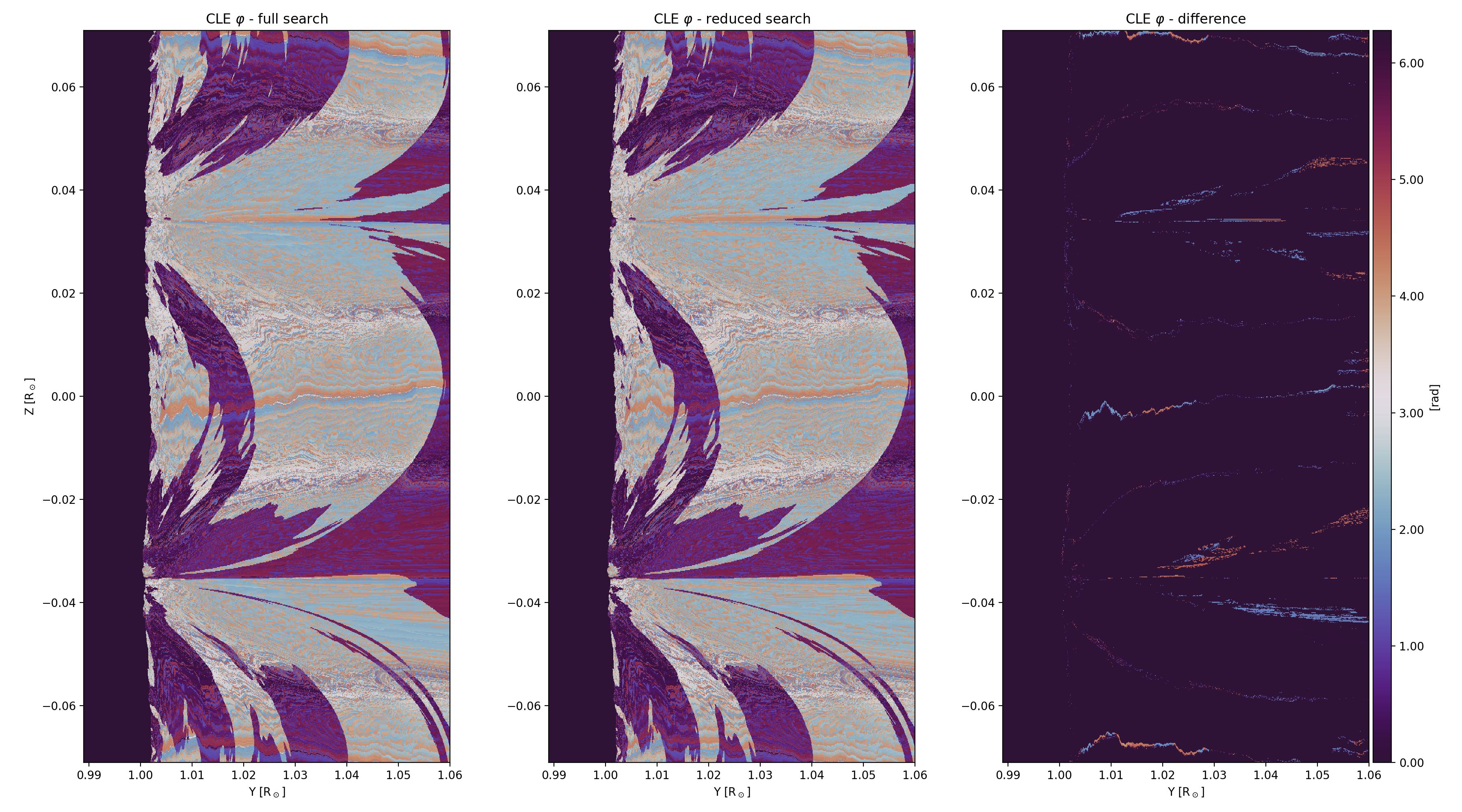
reduced [] booleanParameter to reduce the database size before searching for solutions by using the linear polarization measurements. Dimensionality of db is reduced by over 2 orders of magnitude, enabling significant speed-ups.
Warning
Below figure shows that the solution ordering, or even systematic differences might be altered in certain circumstances when compared to a full search. This is occurring predominantly near field component reversals and around Van-Vleck loci where meaningful solutions are harder to recover. 98% of pixels are not affected. Needlessly, even in the affected areas, the angle differences are modulo 2:math:pi, and thus the basic geometrical orientation would not be significantly altered.
iqud [] booleanSwitches the main matching function of
CLEDB_PROCin order to utilize either Stokes V or Doppler oscillations to compute the magnetic field strength and orientation.
Numba Jit Parameters
jitparallel [] booleanWhen Jit is enabled (jitdisable == False), it controls whether parallel loop-lifting allocations are requested, as opposed to just optimize the execution in single-thread-mode.
jitcache [] booleanJit caching for slightly faster repeated execution. Enable only after no changes to @jit or @njit functions are required. Otherwise kernel restarts are needed to clear caches.
jitdisable [] booleanDebug parameter to control the enabling of Numba Just in Time compilation (JIT) decorators throughout. Higher level verbosity requires disabling the JIT decorators. This functionality can only be done via Numba GLOBAL flags that need to be written to a configuration file
.numba_config.yaml. Any change of this parameter requires a kernel restart.
Constants constants.py Class
## -*- coding: utf-8 -*-
## """
## @author: Alin Paraschiv
##
## """

class Constants:
    """
    A class that defined and transports constants to inversion modules

    Two sets of constants are loaded. General physical constants and ion specific constants based on the specific line requiested.

    To load the class:
    $consts=Constants()
    $print(vars(consts))
    $print(consts.__dict__)

    Attributes:
    -----------
    ion (string): The specific spectroscopic line to load. The individual accepted strings are:
                fe-xiii_1074
                fe-xiii_1079
                si-x_1430
                si-ix_3934
    """
    def __init__(self,ion):
        """
        Main constants initialization function.
        """
        ## Solar units in different projections
        #self.solar_diam_arc = 1919
        #self.solar_diam_deg = self.solar_diam_arc/3600.
        #self.solar_diam_rad= np.deg2rad(0.0174533self.solar_diam_deg)
        #self.solar_diam_st = 2.*np.pi*(1.-np.cos(self.solar_diam_rad/2.))

        ##Physical constants
        self.l_speed       = 2.9979e+8                     ## speed of light [m s^-1]
        self.kb            = 1.3806488e-23                 ## Boltzmann constant SI [m^2 kg s^-2 K^-1];
        self.e_mass        = 9.10938356e-31                ## Electron mass SI [Kg]
        self.e_charge      = 1.602176634e-19               ## Electron charge SI [C]
        self.bohrmagneton  = 9.274009994e-24*1.e-4         ## Bohr magneton [kg⋅m^2⋅s^−2 G^-1]; Mostly SI; T converted to G;
        self.planckconst   = 6.62607004e-34                ## Planck's constant SI [m^2 kg s^-1];

        # ion/line specific constants
        if (ion == "fe-xiii_1074"):
            self.ion_temp = 6.22                      ## Ion temperature SI [K]; li+2017<--Chianti
            self.ion_mass = 55.847*1.672621E-27       ## Ion mass SI [Kg]
            self.line_ref = 1074.6153                 ## CLE/pycelp Ion referential wavelength [nm]
            #self.line_ref = 1074.68                   ## Ion referential wavelength [nm]
            self.width_th = self.line_ref/self.l_speed*(4.*0.69314718*self.kb*(10.**self.ion_temp)/self.ion_mass)**0.5   ## Line thermal width
            self.F_factor= 0.0                             ## Dima & Schad 2020 Eq. 9
            self.gu = 1.5                                  ## upper level g factor
            self.gl = 1                                    ## lower level g factor
            self.ju = 1                                    ## upper level angular momentum
            self.jl = 0                                    ## lower level angular momentum
            self.g_eff=0.5*(self.gu+self.gl)+0.25*(self.gu-self.gl)*(self.ju*(self.ju+1)-self.jl*(self.jl+1))    ## LS coupling effective Lande factor; e.g. Landi& Landofi 2004 eg 3.44; Casini & judge 99 eq 34

        elif (ion == "fe-xiii_1079"):
            self.ion_temp = 6.22                      ## Ion temperature SI [K]; li+2017<--Chianti
            self.ion_mass = 55.847*1.672621E-27       ## Ion mass SI [Kg]
            self.line_ref = 1079.7803                 ## CLE/pycelp Ion referential wavelength [nm]
            #self.line_ref = 1079.79                   ## Ion referential wavelength [nm]
            self.width_th = self.line_ref/self.l_speed*(4.*0.69314718*self.kb*(10.**self.ion_temp)/self.ion_mass)**0.5  ## Line thermal width
            self.F_factor= 0.0                        ## Dima & Schad 2020 Eq. 9
            self.gu = 1.5                             ## upper level g factor
            self.gl = 1.5                             ## lower level g factor
            self.ju = 2                               ## upper level angular momentum
            self.jl = 1                               ## lower level angular momentum
            self.g_eff=0.5*(self.gu+self.gl)+0.25*(self.gu-self.gl)*(self.ju*(self.ju+1)-self.jl*(self.jl+1))    ## LS coupling effective Lande factor; e.g. Landi& Landofi 2004 eg 3.44; Casini & judge 99 eq 34

        elif (ion == "si-x_1430"):
            self.ion_temp = 6.15                      ## Ion temperature SI [K]; li+2017<--Chianti
            self.ion_mass = 28.0855*1.672621E-27      ## Ion mass SI [Kg]
            self.line_ref = 1430.2231                 ## CLE Ion referential wavelength [nm] ;;needs to be double-checked with most current ATOM
            #self.line_ref = 1430.10                   ## Ion referential wavelength [nm]
            self.width_th = self.line_ref/self.l_speed*(4.*0.69314718*self.kb*(10.**self.ion_temp)/self.ion_mass)**0.5  ## Line thermal width
            self.F_factor= 0.5                        ## Dima & Schad 2020 Eq. 9
            self.gu = 1.334                           ## upper level g factor
            self.gl = 0.665                           ## lower level g factor
            self.ju = 1.5                             ## upper level angular momentum
            self.jl = 0.5                             ## lower level angular momentum
            self.g_eff=0.5*(self.gu+self.gl)+0.25*(self.gu-self.gl)*(self.ju*(self.ju+1)-self.jl*(self.jl+1))    ## LS coupling effective Lande factor; e.g. Landi& Landofi 2004 eg 3.44; Casini & judge 99 eq 34

        elif (ion == "si-ix_3934"):
            self.ion_temp = 6.05                      ## Ion temperature SI [K]; li+2017<--Chianti
            self.ion_mass = 28.0855*1.672621E-27      ## Ion mass SI [Kg]
            self.line_ref = 3926.6551                 ## CLE Ion referential wavelength [nm] ;;needs to be double-checked with most current ATOM
            #self.line_ref = 3934.34                   ## Ion referential wavelength [nm]
            self.width_th = self.line_ref/self.l_speed*(4.*0.69314718*self.kb*(10.**self.ion_temp)/self.ion_mass)**0.5  ## Line thermal width
            self.F_factor= 0.0                        ## Dima & Schad 2020 Eq. 9
            self.gu = 1.5                             ## upper level g factor
            self.gl = 1                               ## lower level g factor
            self.ju = 1                               ## upper level angular momentum
            self.jl = 0                               ## lower level angular momentum
            self.g_eff=0.5*(self.gu+self.gl)+0.25*(self.gu-self.gl)*(self.ju*(self.ju+1)-self.jl*(self.jl+1))    ## LS coupling effective Lande factor; e.g. Landi& Landofi 2004 eg 3.44; Casini & judge 99 eq 34
        else:
            print("Not supported ion or wrong string. Ion not Fe fe-xiii_1074, fe-xiii_1079, si-x_1430 or si-ix_3934.\nIon specific constants not returned!")
Python class that unpacks physical constants needed during the inversion. The constants are mainly utilized by the SPECTRO_PROC and BLOS_PROC modules. Ion specific and general atomic and plasma constant parameters are packed herein. The class self-initializes for each requested ion providing its ion specific parameters in a dynamic fashion.
Physical Constants
solar_diam [float*4]Solar diameter in arcsecond, degrees, radians, and steradian units.
l_speed [] floatSpeed of light; Units in SI [m s\(^{-1}\)]
kb [] floatBoltzmann constant; Units in SI [m\(^{-2}\) kg s\(^{-2}\) K\(^{-1}\)]
e_mass [] floatElectron mass; Units in SI [Kg]
e_charge [] floatElectron charge; Units in SI [C]
planckconst [] floatPlanck’s constant; Units in SI [m\(^{-2}\) kg s\(^{-1}\)]
bohrmagneton [] floatBohr Magneton; Units in mostly in SI. T converted to Gauss units [kg m\(^{-2}\) s\(^{-2}\) G\(^{-1}\)]
Ion Specific Constants
Note
Four sets of these constants are provisioned for the four possible lines to invert.
ion_temp [] floatIon temperature; Units in SI [K]
ion_mass [] floatIon mass; Units in SI [Kg]
line_ref [] floatTheoretical line core wavelength position; Units in [nm]
Caution
Simulation examples might have different set line centers based on the spectral synthesis code used. Doppler shift products might not compute correctly.
width_th [] floatThermal width analytical approximation; Units in [nm]
F_factor [] floatAdditional factor described by Dima & Schad, ApJ, 2020. Useful when calculating LOS products in the
BLOS_PROCmodulegu and gl [] floatLS coupling atomic upper and lower energy levels factors
ju and jl [] floatAtomic upper and lower level angular momentum terms
g_eff [] floatLS coupling effective Land\(\acute{e}\) g factor