CLEDB_PROC - Analysis and Inversion

Purpose:

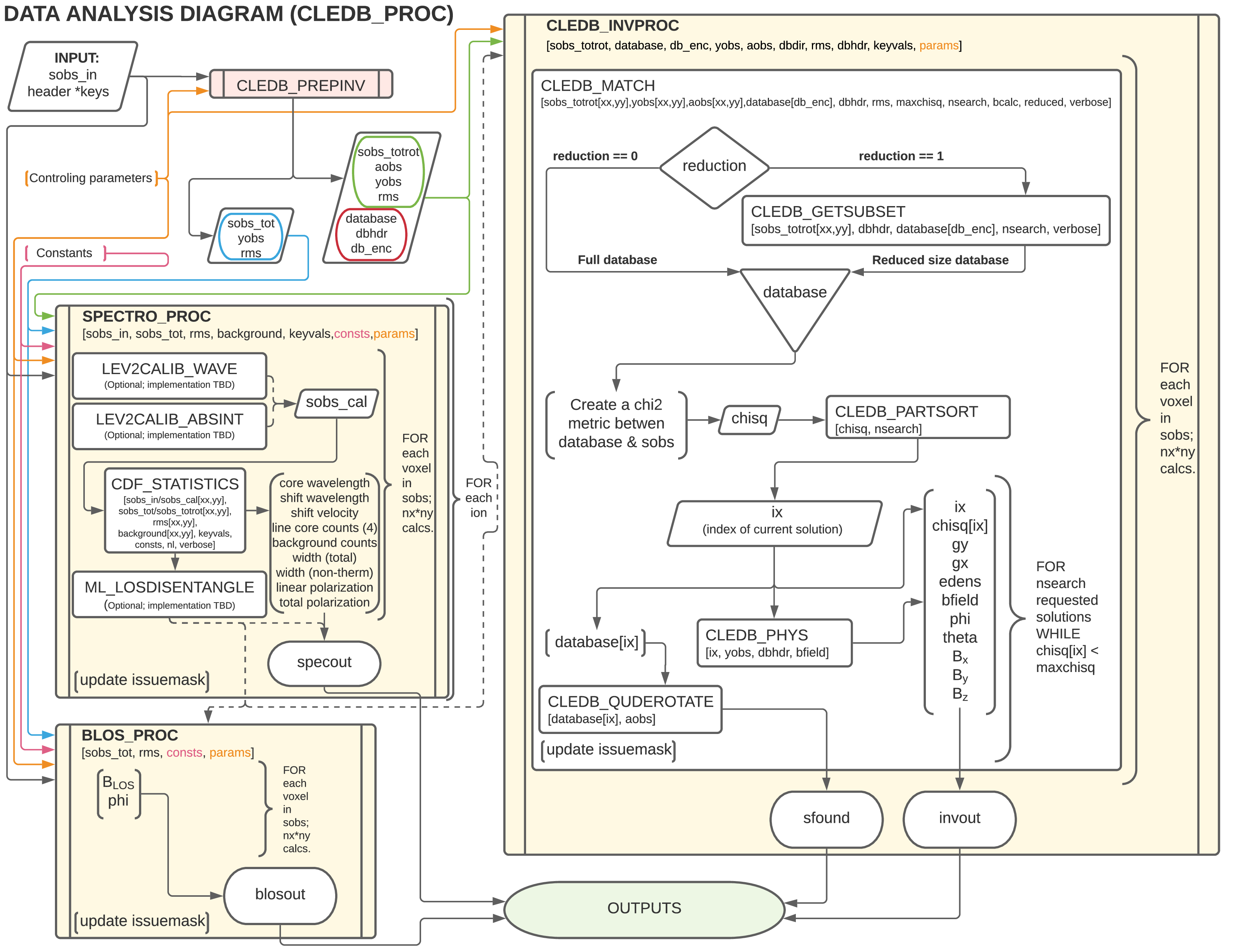
Three main functions, SPECTRO_PROC, BLOS_PROC, and CLEDB_INVPROC are grouped under the CLEDB_PROC data analysis and inversion module. Based on the 1-line or 2-line input data, two or three modules are called. Line of sight or full vector magnetic field outputs along with plasma, geometric and spectroscopic outputs are inverted here. The algorithm flow and a data processing overview is described in the flowchart.

The SPECTRO_PROC Function

Purpose:

Ingests the fully prepped data from sobs_preprocess and produces spectroscopic outputs for each input line. Part of the outputs are used downstream in BLOS_PROC or CLEDB_INVPROC. This module requires data in the formats as resulting from the CLEDB_PREPINV module. Optional sub-modules are envisioned to be integrated into this processing based on upstream instrument processing and retrieved data quality. This is a computationally demanding and time consuming function.

Note

The \(\diamond\), \(\triangleright\), and \(\triangleright\triangleright\) symbols respectively denote main, secondary, and tertiary (helper) level functions. Main functions are called by the example scripts. Secondary functions are called by the main functions, and tertiary from either main or secondary functions.

SPECTRO_PROC Main Functions

\(\diamond\) SPECTRO_PROC

\(\triangleright\) CDF_STATISTICS

Performs pixelwise analysis on the stokes IQUV spectra for each line and computes relevant spectroscopic outputs (see specout) by using via a ctrlparams gaussfit key. By default a gaussian fitting coupled with non-parametric approaches, namely the analysis of CDF functions is utilized.

\(\triangleright\triangleright\) OBS_CDF and ` OBS_GAUSSFIT

These are two helper routines used by CDF_STATISTICS to perform parameter fits and estimations.

Hint

The ctrlparams gaussfit key == 2 represents the slowest component of the entire CDF_STATISTICS block. On the other hand, it is the most accurate and reliable profile fitting method of the three options.

\(\triangleright\) ML_LOSDISENTANGLE (Opt.)

Provisioned to be implemented at a later time. If observations permit, uses Machine Learning techniques for population distributions to help disentangling multiple emitting structures along the LOS in situations where the single point assumption might fail.

\(\triangleright\) LEV2CALIB_WAVE (Opt.)

Provisioned to be implemented at a later time. Higher order wavelength calibration using the spectroscopic profiles. See Ali, Paraschiv, Reardon, & Judge, ApJ, 2022 for additional details. This function can couple if the upstream wavelength accuracy of the input observation is lower than 0.005 nm.

Important

Upstream Level-1 calibration for DKIST is provisioned to match or exceed this accuracy requirement. Implementation is of low priority.

\(\triangleright\) LEV2CALIB_ABSINT (Opt.)

To be implemented at a later time, if feasible. Absolute intensity calibration function that produces an additional output, the calibrated intensity in physical units. The approach is not easily automated as it requires a more convoluted and specific planning of the observations to gather the necessary input data.

Important

This functions was provisioned in the incipient stages of the pipeline design. Subsequently, it was found that CLEDB can utilize only normalized Stokes profiles such that absolute calibrations are not required (see Paraschiv & Judge, SolPhys, 2022). Implementation is halted at this time.

SPECTRO_PROC Main Variables

sobs_cal [nx,ny,sn,4] float array (opt.)

Optional calibrated level-2 data in intensity and or wavelength units. This array would be used by the CDF_STATISTICS function instead of sobs_in.

Note

As LEV2CALIB_ABSINT and LEV2CALIB_WAVE are not currently implemented, sobs_cal is currently just a placeholder.

specout [nx,ny,nline,12] output float array

Returns 12 spectroscopic output products, for each nline input line and for every pixel location.

• specout[:, :, :, 0]

  Wavelength position of the line core. Units are [nm].

• specout[:, :, :, 1]

  Doppler shift with respect to the theoretical line core defined in the constants class line_ref key. Units are [nm].

• specout[:, :, :, 2]

  Doppler shift with respect to the theoretical line core defined in the constants class line_ref key. Units are [km s\(^{-1}\)].

• specout[:, :, :, 3:6]

  Intensity at computed line center wavelength (specout[:, :, :, 0]) for Stokes I, Stokes Q and U. Units are ADU or calibrated physical units if LEV2CALIB_ABSINT is utilized.

• specout[:, :, :, 6]

  Intensity at lobe maximum for Stokes V. The signed “core” counts are measured in the core of the absolute strongest lobe. Thus, the Stokes V measurement will not match the wavelength position of the Stokes IQU intensities. Units are ADU or calibrated physical units if LEV2CALIB_ABSINT is utilized.

  Attention

  If the ctrlparams class iqud key == True, this dimension will be returned implicitly as 0.

• specout[:, :, :, 7]

  Averaged background intensity outside the line profile for the Stokes I component. Since background counts are in theory independent of the Stokes measurement, we utilize just this one realization. Units are ADU or calibrated physical units if LEV2CALIB_ABSINT is used.

• specout[:, :, :, 8]

  Total line FWHM. Units are [nm].

• specout[:, :, :, 9]

  Non-thermal component of the FWHM line width. A measure or estimation of the instrumental line broadening/width will significantly increase the accuracy of this determination. Units are [nm].

  Attention

  Sporadic pixels close to limb in synthetic data exhibited very narrow profiles but otherwise they were deemed usable by the statistics tests. This turns into a problem that will throw invalid value runtime warnings when computing this quantity. To fix, we set specout[:, :, :, 9] = 0 in all such occurences.

• specout[:, :, :, 10]

  Fraction of linear polarization P_l with respect to the total Stokes I counts. Dimensionless.

• specout[:, :, :, 11]

  Fraction of total polarization (linear + circular) P_v with respect to the total Stokes I counts. Dimensionless.

Attention

Regardless if solving for 1-line or 2-line observations, specout will return both nline dimensions. In the case of 1-line observations, the nline = 1 dimension corresponding to the hypothetical second line is returned as 0 for all pixel locations. The unused dimension can be removed from the upstream example script, if needed. This behavior is known and enforced to keep output casting static, making the codebase compatible with Numba and speeding up execution.

The BLOS_PROC Function

Error

Stokes V observations are required for this analytical method. Thus, BLOS_PROC is incompatible with the IQUD setup.

Purpose:

Implements the analytical solutions of Casini & Judge, ApJ, 1999 and Dima & Schad, ApJ, 2020 to calculate the LOS projected magnetic field strength and magnetic azimuth angle. The module returns two degenerate constrained magnetograph solutions, where the one that matches the sign of the atomic alignment is more precise. The less precise “classic” magnetograph formulation is also returned.

Attention

There is not enough information in 1-line observations to deduce which of the two degenerate solution is “more precise”. The “classic” magnetograph estimation is less precise than the optimal degenerate constrained magnetograph solution, but more precise than the other. The differences will vary from insignificant to tens of percents of the magnetic field strength based on observation and magnetic geometry, and degree of linear polarization. The choice of what product to use remains the prerogative of the user.

This branch requires only 1-line observations (4 stokes profiles). The setup is used to get as much magnetic information as possible (the field strength and LOS projection) in the absence of a second line. For a sobs_tot input of 2-lines, the module will produce independent products for each input line observation.

Hint

Observations of Si X 1430.10 nm will benefit from an additional alignemnt correction due to the non-zero F factor of this transition. Additional details in Dima & Schad, ApJ, 2020.

BLOS_PROC Main Functions

\(\diamond\) BLOS_PROC

BLOS_PROC Main Variables

blosout [nx,ny,4*nline] output float array

The array returns 4 or 8 products containing LOS projected magnetic field estimations and magnetic azimuth angle in G units at each pixel location.

• blosout[:, :, 0] and/or blosout[:, :, 4]

  First degenerate constrained magnetograph solution for each respective line.

• blosout[:, :, 1] and/or blosout[:, :, 5]

  Second degenerate constrained magnetograph solution for each respective line.

• blosout[:, :, 2] and/or blosout[:, :, 6]

  “Classic” magnetograph solution for each respective line. Values lie in between the two above degenerate solutions.

• blosout[:, :, 3] and/or blosout[:, :, 7]

  Magnetic field azimuth angle derived from the Q and U linear polarization components of the respective line; -\(\pi\) to \(\pi\) range.

Warning

A \(\frac{\pi}{2}\) degeneracy will manifest due to using arctan functions to derive the angle.

The CLEDB_INVPROC Function

Purpose:

Main 2-line inversion function. CLEDB_INVPROC compares the preprocessed observations with the selected databases by performing a \(\chi^2\) goodness of fit measurement between each independent voxel and the complete set of calculations in the matched database. If CLEDB_GETSUBSET is enabled via ctrlparams class getsubset key, a presorting of the database entries to those that match the direction of observer linear polarization azimuth is performed. After the main sorting is performed, the best database solutions are then queried with respect to the physical parameters that gave the matched profiles. CLEDB_INVPROC acts like a pixel iterator and variable ingestion setup for either CLEDB_MATCHIQUV or CLEDB_MATCHIQUD.

Caution

The reduced presorting will slightly change the final ordering of solutions in certain cases.

CLEDB_INVPROC Main Functions

\(\diamond\) CLEDB_INVPROC

\(\diamond\) CLEDB_MATCHIQUV

Matches a set of two full Stokes IQUV observations with a model observation of the same Stokes quantities. Solutions are 2 times degenerate with respect to the LOS. Matching is done individually for one pixel in the input array. This is a computationally demanding and time consuming function.

\(\diamond\) CLEDB_MATCHIQUD

Matches a set of two partial Stokes IQU observations with a model observation of the same Stokes quantities. The matched solutions are initially more degenerate than CLEDB_MATCHIQUV, usually 4 timee with respect to LOS and signed field strength combinations. We are currently evaluating the feasibility of including additional information from Doppler oscillation tracking to recover field strengths and reduce degeneracies (to 2 times). Matching is done individually for one pixel in the input array. This is a computationally demanding and time consuming function.

Note

Based on the ctrlparams iqud key only one of the CLEDB_MATCHIQUV or CLEDB_MATCHIQUD setups is selected and utilized.

\(\triangleright\) CLEDB_GETSUBSETIQUV

When enabled via ctrlparams, the information encoded in the Stokes Q and U magnetic azimuth is used to reduce the matched database by approximately 1 order of magnitude in terms of observation-comparable calculations.

\(\triangleright\) CLEDB_GETSUBSETIQUD

When reduced is enabled via ctrlparams, the information encoded in the doppler wave angle azimuth is used to reduce the matched database by approximately 1 order of magnitude in terms of observation-comparable calculations.

Attention

Tests done on CoMP and uCoMP data showed that when Doppler oscialtions are avaialble, using the phase angle as a proxy (as opposed to the default linear polarization azimuth) for running reduced runs, produces a more sharp output with better details especially around regions where magnetic polarity reverses. CLEDB_GETSUBSETIQUD will use this information if available. This option can not be directly enabled for IQUV matches yet, as the doppler oscilation data requires special observing conditions and separate processing. Some altering of matching and subset selecting functions by the user will be required to enable such a setup.

Important

If the subset calculation is enabled via ctrlparams, execution time in the case of large databases is significantly decreased.

\(\triangleright\) CLEDB_PARTSORT

A custom function that performs a fast partial sort of the input array because only a small subset of ctrlparams nsearch key solutions are requested via the ctrlparams nsearch key. This increases execution times by a few factors when requesting just few nsearch solutions (< 100 on 10\(^8\) entries databases). CLEDB_PARTSORT is used by CLEDB_MATCHIQUV, CLEDB_MATCHIQUD, and CLEDB_GETSUBSET functions. In CLEDB_MATCH, CLEDB_PARTSORT performs a < nsearch sorting of database entries based on the \(\chi^2\) metric. In CLEDB_GETSUBSET, CLEDB_PARTSORT selects for each \(\varphi\) angle orientation only the most compatible \(\vartheta\) directions based on the \(\Phi_B\) azimuth given by the linear polarization Q and U measurements.

\(\triangleright\) CLEDB_PHYS

Returns 9 physical and geometrical parameters corresponding to each selected database index following the ctrlparams nsearch and maxchisq constraints. These products are returned as dimensions of the invout output variable.

\(\triangleright\triangleright\) CLEDB_PARAMS, CLEDB_INVPARAMS, CLEDB_ELECDENS, and CLEDB_PHYSCLE

These are helper functions that prop CLEDB_PHYS by providing interfaces with the parameters encoded in selected databases and helping transform quantities between different geometrical systems.

\(\triangleright\) CLEDB_QUDEROTATE

The inverse function of OBS_QUROTATE. Derotates the Q and U components from each selected database entry, in order to make the set of fitted solutions directly comparable with the original integrated input sobs_tot observation.

CLEDB_INVPROC Main Variables

database [ned,nx,nbphi,nbtheta,nline*4] list of float arrays

Individual entries from the database list are fed to the CLEDB_MATCHIQUV or CLEDB_MATCHIQUD functions. From the database list, only the best matching height entry via db_enc variable is passed via the database_in internal variable.

database_sel [ned,nx,nbphi,nbtheta,nline*4] float array

An element reduced database list that is used by CLEDB_MATCHIQUV or CLEDB_MATCHIQUD for matching the observation in one pixel. This alleviates memory shuffling and array slicing operations. The array is reshaped into a 2D [ned*nx*nbphi*nbtheta,nline*4] form (e.g. [index,nline*4]). In the case where ctrlparams reduction key is enabled, database_sel is additionally reduced with respect to the number of potential indexes to match. Otherwise, the variable is only trimmed of the entries where the sign of Stokes V does not math the observation.

sobs_totrot

Input variable to CLEDB_INVPROC described here.

sobs_dopp

Doppler oscillation magnetic field strength and POS orientation resulting from Doppler oscillation analysis. The two utilized dimensions are sobs_dopp[:,:,0] and sobs_dopp[:,:,1] representing respectively the magnetic field strength and the wave angle. The two other dimensions represent POS projections of the magnetic field computed either via the linear polarization azimuth or the afore mentioned wave angle, but are not currently utilized.

Caution

sobs_dopp is only used as input to CLEDB_MATCHIQUD when ctrlparams iqud is enabled. For Numba consistency, an empty array is also passed to CLEDB_INVPROC when performing full IQUV inversions, but it is never used.

chisq [ned*nx*nbphi*nbtheta,nline*4] float array

Computes the squared difference between the voxel IQUV measurements [nline*4] and each index element of the database [index,nline*4].

sfound [nx,ny,nsearch,nline*4] output float array;

Returns the first nsearch de-rotated and matched Stokes IQUV sets from the database. These can be compared to the input Stokes observation.

Caution

As the databases are only computed for B = 1 G, the Stokes V profiles will not match accurately. The sign should match.

invout [nx,ny,nsearch,11] output float array

Main 2-line inversion output products. invout contains the matched database index, the \(\chi^2\) fitting residuals, and 9 inverted physical parameters, for all nsearch closest matching solutions with respect to the input observation. The 11 parameters follow with individual descriptions.

• invout[:,:,:,0]

  The index of the database entry that was matched at the nsearch rank. The index is used to retrieve the encoded physics that match the observations.

• invout[:,:,:,1]

  The \(\chi^2\) residual of the matched database entry.

• invout[:,:,:,2]

  Plasma density computed via the database. This output is applicable for the Fe XIII 1074.68/1079.79 line ratio (same ion). Other line combinations will produce less accurate results due to the relative abundance ratios, that are varying dynamically. For a real-life observation, we do not consider trustworthy the implicit static relative abundance ratios of different ions, resulted from the CHIANTI tabular data implicitly ingested via the ATOM files when build databases. Units are logarithm of number electron density in cm\(^{-3}\).

• invout[:,:,:,3]

  The apparent height of the observation. Analogous to the yobs variable. Units are R\(_\odot\).

• invout[:,:,:,4]

  Position of the dominant emitting plasma along the LOS. Units are R\(_\odot\).

• invout[:,:,:,5]

  Magnetic field strength recovered via the ratio of observed stokes V to database Stokes V (computed for B = 1 G); Uses ctrlparams class bcalc key. Units are [G].

  Warning

  Due to how the problem is posed, CLEDB_MATCHIQUV can only use bcalc = 0, 1, or 2 while CLEDB_MATCHIQUD can only use bcalc = 3.

  Attention

  The bcalc estimation employs a logical test to avoid division by 0 in cases where the Zeeman signal vanishes due to geometry in teh database. If the database Stokes V component is less than 1e-7, then the matched field strength is set to 0 regardless of what the signal is in the observation(usually it is very small, or noise)

• invout[:,:,:,6]

  Magnetic field \(\varphi\) LOS angle in CLE frame. Range is 0 to \(2\pi\).

• invout[:,:,:,7]

  Magnetic field \(\vartheta\) POS Azimuth angle in CLE frame. Range is 0 to \(\pi\).

• invout[:,:,:,8]

  B_x cartesian projected magnetic field depth/LOS component. Units are [G].

• invout[:,:,:,9]

  B_y cartesian projected magnetic field horizontal component. Units are [G].

• invout[:,:,:,10]

  B_z cartesian projected magnetic field vertical component. Units are [G].

Warning

• Solutions are skipped if the \(\chi^2\) fitting residuals are greater than the limit set by the ctrlparams maxchisq key. Thus, it is possible and even expected that less than requested ctrlparams nsearch solutions to be returned for one observed voxel in both invout and sfound.

• Regardless of the number of solutions (if any) that are found inside the ctrlparams maxchisq and nsearch constraints, the invout output array will keep its dimensions fixed and return “0” value fields to keep output data shapes consistent. This is a Numba requirement. Only the index is set to “-1” to notify the user that no result was outputted. sfound behaves similarly.